Slaves of some defunct economist
April 2, 2022 – Weekly comment
Challenge of Central Banking in a Democratic Society- Dec 1996 – Irrational Exuberance speech
…The stagflation of the 1970s required a thorough conceptual overhaul of economic thinking and policymaking. Monetarism, and new insights into the effects of anticipatory expectations on economic activity and price setting, competed strongly against the traditional Keynesianism. Gradually the power of state intervention to achieve particular economic outcomes came to be seen as much more limited. A consensus gradually emerged in the late 1970s that inflation destroyed jobs, or at least could not create them.
But where do we draw the line on what prices matter? Certainly prices of goods and services now being produced–our basic measure of inflation–matter. But what about futures prices or more importantly prices of claims on future goods and services, like equities, real estate, or other earning assets? Are stability of these prices essential to the stability of the economy?
…how do we know when irrational exuberance has unduly escalated asset values, which then become subject to unexpected and prolonged contractions
Jackson Hole Speech – August 1999
History tells us that sharp reversals in confidence happen abruptly, most often with little advance notice. These reversals can be self-reinforcing processes that can compress sizable adjustments into a very short time period. Panic market reactions are characterized by dramatic shifts in behavior to minimize short-term losses. Claims on far-distant future values are discounted to insignificance. What is so intriguing is that this type of behavior has characterized human interaction with little appreciable difference over the generations. Whether Dutch tulip bulbs or Russian equities, the market price patterns remain much the same.
Collapsing confidence is generally described as a bursting bubble, an event incontrovertibly evident only in retrospect. To anticipate a bubble about to burst requires the forecast of a plunge in the prices of assets previously set by the judgments of millions of investors, many of whom are highly knowledgeable about the prospects for the specific companies that make up our broad stock price indexes.
As we make progress, hopefully, toward understanding asset-pricing mechanisms, we need also to upgrade our insights into the effect of changing asset values on GDP–the so-called wealth effect.
In conclusion, the issues that I have touched on this morning are of increasing importance for monetary policy. We no longer have the luxury to look primarily to the flow of goods and services, as conventionally estimated, when evaluating the macroeconomic environment in which monetary policy must function. There are important–but extremely difficult–questions surrounding the behavior of asset prices and the implications of this behavior for the decisions of households and businesses. Accordingly, we have little choice but to confront the challenges posed by these questions if we are to understand better the effect of changes in balance sheets on the economy and, hence, indirectly, on monetary policy.
Alan Greenspan’s speeches were thought-provoking. He was Fed Chair from August 1987 until January 2006. He was clearly intrigued by the interplay of asset prices, confidence, trust, and their effect on the performance of the economy. During his tenure the Fed navigated the 1987 stock crash, the Russian devaluation, the SE Asia crisis, the dotcom bubble, 9/11, and several rate hike cycles.
In the top line of this note Greenspan says “the power of state intervention to achieve particular economic outcomes came to be seen as much more limited.” The next sentence implicitly links excessive gov’t spending with inflation which leads to job destruction. We’ve now swung the pendulum to the opposite end of the spectrum with MMT, but clearly the first outcome of state intervention has occurred, i.e. inflation, even though the lagging indicator of unemployment has just notched a near record low of 3.6%. (Of course, intervention due to covid was essential, but the extraordinary stimulus of the Fed’l Gov’t and Fed sparked inflation).
There are now many comparisons being made with the 1994 hiking cycle. Throughout 1993 Fed Funds were 3%. 1994 started with a 2y note yield of just over 4%, and CPI at 2.5 to 2.6%. I.e. real rates were positive. In Jan 1995, FF peaked at 6%, a total increase of 300 bps; a double. At the end of 1994, the 2y yield topped at just under 7.75%, not quite a double, a move of 375 bps. Over this period CPI peaked in Sept’94 at 3%, fell back a bit, and then ultimately rose to 3.2% by Q2 1995 before ending that year at 2.6%.
This is NOT 1994. FF started this year at 0-0.25%. The 2y started at 75 bps, and CPI began 2022 at 7%. In 1994 Fed’l Debt to GDP was just under 68%, now it’s over 120%. In 1994 the ‘Buffet Indicator’ of market cap to GDP was also around 68%, now it’s 202%. The 2yr yield was 58 bps at the end of November. In four months it has surged to 244 bps, a change of 186 bps, about half the 1994 move in a third of the time. Of course in percentage terms the move is much more dramatic. The rapid adjustment in short end rates is nothing less than a shock to the economic system.
Let’s return to Greenspan’s concern with the wealth effect. With total Net Worth reported to be a record $150 trillion as of the end of 2021, and market cap to GDP also near a record 200%, and the Shiller p/e ratio currently at 37 (vs long-term mean of 17 and an all time peak of 44 in 1999’s dotcom mania), could a crack in confidence cause a rapid re-pricing of financial assets?
How can we tell if confidence is starting to fray? Consumer confidence surveys. Presidential approval ratings. Spreads on riskier securities. Borrowings. The chart below shows University of Mich Consumer Sentiment (red), the Conference Board’s Confidence measure (white) and the NFIBs Small Business Optimism (green). All have turned down. UofM is close to the GFC low, and it appears from the experience in 2007 that UofM leads the others.
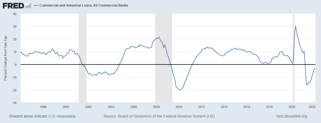
I have also included a chart of the yoy percent change in Commercial and Industrial Loans, last at -3.9% (Feb). Obviously there was a surge in 2020 as companies drew down credit lines. It’s only natural that these emergency loans are paid back or forgiven. But it’s still a net reversal of economic liquidity at the same time as a shift in the Fed’s stance. In a speech yesterday, NY Fed’s Williams said a reduction in the Fed’s balance sheet could begin as soon as the next FOMC in May. I suspect the withdrawal of liquidity will negatively impact confidence in the system.
In my opinion, there is one more measure of confidence that impacts asset values: the yield curve. This week the most popular measure, 2/10 spread, flipped from positive 19.3 to negative 5.5 (partially impacted by new 2yr). Even the 2y to 30y ended the week slightly inverted. And of course, the red Eurodollar pack (2nd year forward) to greens, blues and golds (3rd, 4th and 5th years forward) hit historic new lows. The reds ended with a yield of approx. 3.24%, greens at 2.89%, blues 2.52% and golds 2.36%.
What does this mean? It’s clear why the reds have plummeted in price to new high yields, the Fed is expected to aggressively raise short term rates. Why are yields on more deferred years lower? Because the market doesn’t think the economy can withstand the shock of higher funding costs. Funding costs will overwhelm returns on longer dated assets. It is a measure of forward confidence. That’s why the curve is a recession indicator. I don’t know why the press continues to quote people that say it’s debatable as to whether an inverted curve signals recession. It does. I’m not saying that market pricing can’t change, and with it, the signal. For example, the Ukraine conflict could end, China’s property slump could magically abate, and the supply chain could revert to smooth functioning.
The capitalistic monetary system borrows short and lends long. That’s the financial transformation through which savers fund enterprises leading to increases in standards of living. Emergency government injections of funds saved a lot of jobs and businesses, but subsequently led to a lot of bad decisions based on hope. The reaction is here. If funds can’t be borrowed profitably, growth declines.
OTHER MARKET THOUGHTS/ TRADES
EDM’22/EDM’23 calendar settled at a new high for any one-yr during this cycle at 174.5 bps. Peak rates on the curve are EDM’23 at 9668.5 or 3.315%. SFRM3 at 9694.5 or 3.055%. FFU3 at 9689.5 or 3.105%. Therefore, highs for the rate cycle continue to project the middle of next year at a bit over 3%. However, prices were so weak and liquidity so bad on Friday, with reds -18.5 bps, and the 5yr up 12.7 bps to 2.545% that it’s impossible to say where ultimate highs might be on a true washout.
| 3/25/2022 | 4/1/2022 | chg | ||
| UST 2Y | 233.5 | 242.8 | 9.3 | |
| UST 5Y | 257.2 | 254.5 | -2.7 | |
| UST 10Y | 249.0 | 237.3 | -11.7 | |
| UST 30Y | 260.2 | 242.1 | -18.1 | |
| GERM 2Y | -13.5 | -6.8 | 6.7 | |
| GERM 10Y | 58.7 | 55.5 | -3.2 | |
| JPN 30Y | 96.8 | 94.8 | -2.0 | |
| CHINA 10Y | 280.0 | 277.7 | -2.3 | |
| EURO$ M2/M3 | 154.5 | 174.5 | 20.0 | |
| EURO$ M3/M4 | -24.0 | -30.5 | -6.5 | |
| EURO$ M4/M5 | -18.0 | -36.5 | -18.5 | |
| EUR | 109.82 | 110.46 | 0.64 | |
| CRUDE (active) | 113.90 | 99.27 | -14.63 | |
| SPX | 4543.06 | 4545.86 | 2.80 | 0.1% |
| VIX | 20.81 | 19.63 | -1.18 | |
https://www.federalreserve.gov/boarddocs/speeches/1996/19961205.htm
https://www.federalreserve.gov/boarddocs/speeches/1999/19990827.htm